Seto's Page

Switch to

Last update:

Rodrigues Space

On the previous page, we learned the concept of quaternions as one of the representations of rotation, and considered the distribution of angular differences in random orientation states for objects without symmetry other than the identity transformation. Here, we explain the concept of Rodrigues space, another important rotation representation, and introduce the idea of “compression” through rotational symmetry.

What is Rodrigues Space

Three-dimensional Rodrigues space (hereafter simply called Rodrigues space) is a space that represents the direction of the rotation axis and the amount of rotation. A point in this space is represented by three variables, $\textbf{r}=(x,y,z)$. The norm is defined as $ \|\textbf{r}\| = \sqrt{x^2+y^2+z^2}$, and since it appears very frequently, we also define $\rho = \|\textbf{r}\| $. The coordinates $(x,y,z)$ in Rodrigues space mean

The direction of the rotation axis is $(x,y,z)$
The rotation amount $\theta$ is $ 2\arctan(\|\textbf{r}\|) = 2\arctan(\rho) $ (i.e., $\tan\frac{\theta}{2} = \rho$)

For example, the coordinate $ (1,0,0) $ means “rotation of 90 degrees around the X-axis,” and the coordinate $ (1,1,1) $ means “rotation of 120 degrees (=$2\arctan(\sqrt{3})$) around the composite vector of X, Y, Z.”

Rodrigues coordinates ($\textbf{r}$) and the unit quaternions from the previous page ($q$) have the elegant relationships:$$
\textbf{r}=(x,y,z) \quad \leftrightarrow \quad q = \frac{1}{\sqrt{1+x^2+y^2+z^2}}( 1 ,x ,y, z ) =\frac{1}{\sqrt{1+\rho^2}}( 1 ,\textbf{r} ) $$or$$
\textbf{r}=\tan\frac{\theta}{2}(x, y, z) \quad \leftrightarrow \quad q = (\cos\frac{\theta}{2}, x\sin\frac{\theta}{2},y\sin\frac{\theta}{2},z\sin\frac{\theta}{2}) =\cos\frac{\theta}{2}(1, \textbf{r}) \quad \textrm{where}\ x^2+y^2+z^2=1 $$or$$
\textbf{r}=\frac{\textbf{v}}{s} \quad \leftrightarrow \quad q=(s,\textbf{v}) \quad \textrm{where}\ s^2+\|\textbf{v}\|^2=1 $$

Operations in Rodrigues Space

Multiplication of two coordinates in Rodrigues space corresponds to composition of rotations. Let us define two coordinates $\textbf{r}_1, \textbf{r}_2$ in Rodrigues space as
$$\textbf{r}_1=(x_1,y_1,z_1),\quad \textbf{r}_2=(x_2,y_2,z_2)
$$and further define $\rho_1 = \|\textbf{r}_1\|,\ \rho_2 = \|\textbf{r}_2\| $. The corresponding quaternions $q_1, q_2$ are$$
q_1=\frac{1}{\sqrt{1+\rho_1^2}}(1,\,\textbf{r}_1),\qquad q_2=\frac{1}{\sqrt{1+\rho_2^2}}(1,\,\textbf{r}_2)
$$The product of quaternions ($q=q_1q_2$) is, as explained on the previous page, $$
q=q_1q_2=\frac{1}{\sqrt{(1+\rho_1^2)(1+\rho_2^2)}} \left( 1-\textbf{r}_1\cdot \textbf{r}_2,\ \textbf{r}_1+\textbf{r}_2+\textbf{r}_1\times \textbf{r}_2 \right) \\
= \frac{1}{(1-\textbf{r}_1\cdot \textbf{r}_2) \sqrt{(1+\rho_1^2)(1+\rho_2^2)}} (1, \ \frac{\textbf{r}_1+\textbf{r}_2+\textbf{r}_1\times \textbf{r}_2}{1-\textbf{r}_1\cdot \textbf{r}_2})
$$Therefore, the Rodrigues coordinate $\textbf{r}$ obtained from composition of rotations is$$
\textbf{r} = \textbf{r}_1\otimes \textbf{r}_2 = \frac{\textbf{r}_1+\textbf{r}_2+\textbf{r}_1\times \textbf{r}_2}{1-\textbf{r}_1\cdot \textbf{r}_2}
$$where $\otimes$ denotes multiplication in Rodrigues space. As is clear from this equation, when $1-\textbf{r}_1\cdot \textbf{r}_2=0$, the scalar part of the quaternion of the composite rotation becomes 0, and the rotation angle becomes 180 degrees. At this point, the Rodrigues coordinate diverges to $ \rho \to\infty$.

For the inverse element, since quaternions have the conjugate $q^{-1}=q^*$, in Rodrigues space it is simply$$\textbf{r}^{-1}=-\textbf{r}$$The rotation amount (corresponding to the distance from the origin) is the same, but the rotation axis is opposite. As a result, the orientation difference (misorientation) $\Delta$ between two Rodrigues coordinates $\textbf{r}_1,\textbf{r}_2$ is$$\Delta \textbf{r} = \textbf{r}_1^{-1}\otimes \textbf{r}_2 = (-\textbf{r}_1)\otimes \textbf{r}_2 = \frac{-\textbf{r}_1+\textbf{r}_2-\textbf{r}_2\times \textbf{r}_1}{1+\textbf{r}_1\cdot \textbf{r}_2}$$

Distribution of $SO(3)$ in Rodrigues Space

Rodrigues space, like unit quaternions, is a space that represents $SO(3)$, but there is an important caveat. It is that $SO(3)$ is not uniformly distributed in Rodrigues space¹. This is easy to understand from the fact that a 180-degree rotation corresponds to a point at infinity in Rodrigues space. So, with what density is $SO(3)$ distributed in Rodrigues space? In conclusion, this is a problem of calculating the Jacobian for the mapping from uniform distribution on the quaternion $S^3$ to Rodrigues space. The detailed explanation is deferred to the next page², but this density function $P$ is a function of $\rho= \|\mathbf{r})\| $, and its form is $$ P(\rho) = \frac{1}{\pi^2(1+ \rho^2)^2}$$

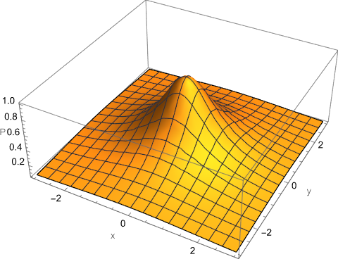
Shape of $P(\rho)$ at $z=0$³

The area of a sphere consisting of point sets at distance $\rho$ from the origin in Rodrigues space is $4\pi\rho^2$, and the $SO(3)$ density on this spherical surface is proportional to $\pi^{-2}(1+\rho^2)^{-2}$, so the orientation difference distribution function $F$ becomes$$F(\rho) = \frac{4\rho^2}{\pi(1+ \rho^2)^2}$$Substituting $ \rho=\tan(\theta/2)$ and rewriting as $F(\theta)$,$$
\frac{d\rho}{d\theta}=\frac{1}{2}(1+\rho^2)\\
F(\theta) = F(\rho)\frac{d\rho}{d\theta} = \frac{2 \rho^2}{\pi(1+ \rho^2)}=\frac{2}{\pi}\frac{\tan^2\frac{\theta}{2}}{1+ \tan^2\frac{\theta}{2}}=\frac{2}{\pi}\sin^2\frac{\theta}{2} = \frac{1-\cos\theta}{\pi}$$which agrees with the formula shown on the previous page.

Compression of Rodrigues Space by Symmetry Elements

Here, we examine how rotational symmetry affects the density function in Rodrigues space.

Case of $2$-fold Rotation

First, as the simplest example, consider 2-fold rotation. The 2-fold rotation operation (180-degree rotation) along the X-axis in Rodrigues space, $\textbf{C}_2$, can be expressed as$$\textbf{C}_2= \lim_{A \to \infty}(A, 0,0)$$By this operation, a point $\textbf{r} =(x,y,z)$ in Rodrigues space is mapped to another point $\textbf{r}’=(u,v,w)$. Applying the rotation composition formula, $\textbf{r}’$ can be expressed as follows:$$
\textbf{r}’ = (u,v,w) = \textbf{C}_2 \otimes \textbf{r} = (-\frac{1}{x},\frac{z}{x},-\frac{y}{x})
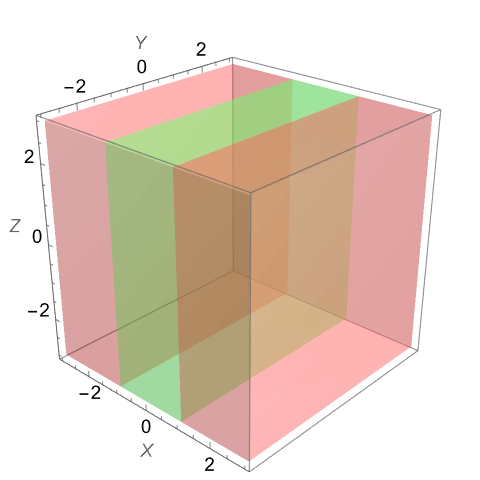
$$Looking at this formula, we can see that when $|x| \ge 1$, we have $|u| \le 1$⁴. That is, as shown in the following figure⁵, the region where $|x| \ge 1$ (red in the figure) is compressed by the symmetry operation into the region where $ |x| \le 1$ (green in the figure), so there is no need to consider it separately.

Now we know that we only need to consider the region $ |x| \le 1$, but the points compressed from $|x| \ge 1$ might disturb the $SO(3)$ density function $P(\rho)$ in the $|x’| \le 1$ region. Let us check this anyway. First, the Jacobian of the transformation $\mathbf{r} \to \mathbf{r}’$ is$$
\det \left[\frac{\partial(u,v,w) }{\partial(x,y,z)}\right] = \frac{1}{x^4}
$$⁶. That is, the rate of change of the infinitesimal volume around each point before and after transformation, $ \large \frac{du\ dv\ dw}{dx\ dy\ dz}$, is $x^{-4}$. On the other hand, the $SO(3)$ distribution density before and after transformation changes from $P(\rho)= \large \frac{1}{\pi^2(1+ \rho^2)^2}$ to $P(\rho’)=\large \frac{1}{\pi^2(1+\rho’^2)^2}$, so the rate of change is$$
\frac{(1+ \rho^2)^2}{(1+ \rho’^2)^2}=
\left(\frac{1+ x^2+y^2+z^2}{1+ \frac{1+y^2+z^2}{x^2} }\right)^2=x^4
$$The infinitesimal volume around a point changes by a factor of $x^{-4}$ due to the transformation, so the density becomes $x^4$ times. However, the change in the density function $P(\rho)$ before and after transformation is already $x^4$ times, so focusing on that part, the density becomes twice. And since there is no overlap in the compression from $|x| \ge 1$ to $ |x| \le 1$, we can conclude that by compressing the entire region $|x| \ge 1$ into it, the density $P(\rho)$ within $ |x| \le 1$ becomes uniformly twice the original value (without the shape being disturbed).

Case of $n$-fold Rotation

Finally, we generalize the order of rotational symmetry to $n$ and show how the density function $P(\rho)$ and the range change due to compression by this symmetry element. Since the choice of rotation axis does not restrict generality, we consider the operation of rotating by angle $\large \frac{2k\pi}{n}$ along the X-axis (where $k$ is an integer from $0$ to $n-1$). When a point $\textbf{r} =(x,y,z)$ in Rodrigues space is mapped to another point $\textbf{r}’=(u,v,w)$ by this operation, with $\theta_k = \large \frac{k\pi}{n}$, the relationship is$$
(u,v,w) = (\frac{x+\tan\theta_k}{1-x\tan\theta_k},\frac{y-z\tan\theta_k}{1-x\tan\theta_k},\frac{z+y\tan\theta_k}{1-x\tan\theta_k})
$$Computing the Jacobian⁷ of this transformation gives $\large \frac {(1+\tan^2\theta_k)^2}{(1-x \tan\theta_k)^4}$. On the other hand, for the density function,$$
P(\rho’) = \left[\frac{1}{\pi(1+u^2+v^2+w^2)}\right]^2 = \left[\frac{(1-x\tan\theta_k)^2} {\pi(1+x^2+y^2+z^2)(1+\tan^2\theta_k)}\right]^2 = P(\rho) \frac{(1-x\tan\theta_k)^4} {(1+\tan^2\theta_k)^2}
$$so, similarly to the 2-fold rotation argument, the density function $P(\rho)$ becomes uniformly multiplied by a constant.

Let us also consider the range into which the points are compressed. Focusing on the X-coordinate, and further substituting $x=\tan\alpha$ ($0 \le \alpha \le \pi/2$), we can use the addition formula for trigonometric functions to obtain $$ u= \frac{x+\tan\theta_k}{1-x\tan\theta_k}=\frac{\tan\alpha+\tan\theta_k}{1-\tan\alpha\tan\theta_k} =\tan(\alpha+\theta_k)=\tan(\alpha+\frac{k\pi}{n})
$$This is a beautiful relationship. Therefore, listing only the X-coordinates of the set of points that are equivalent by $n$-fold rotation along the X-axis, we get$$
\tan(\alpha),\ \tan(\alpha+\frac{\pi}{n}),\ …\ ,\tan(\alpha+\frac{n-2}{n}\pi),\ \tan(\alpha+\frac{n-1}{n}\pi)
$$These are a sequence of the tangent function evaluated at equally spaced angles $\large \frac{\pi}{n}$, so one value must be included in the range $-\tan\frac{\pi}{2n}\sim \tan\frac{\pi}{2n}$. Regarding this as a representative of equivalent points, if we compress all points from $|x|\ge\tan\frac{\pi}{2n}$, then we only need to consider $|x|\le\tan\frac{\pi}{2n}$.

Summarizing the above discussion, we have the following: By $n$-fold rotation along a certain axis, Rodrigues space is compressed into a region sandwiched between two planes with that axis as their normal, and the orientation density function within the region is multiplied by $n$. The two planes are symmetric with respect to the origin, and their distance from the origin is $\tan(\pi/2n)$.

On the next page, we will consider specific point groups and calculate orientation difference distribution functions.

Footnotes

More precisely, the Haar measure is not uniform. As explained on the previous page, $SO(3)$ is uniformly distributed on $S^3$ as unit quaternions. Four dimensions are necessarily required to represent uniform distribution. ↩︎
Intuitively, as shown in the relationship $ r=(x,y,z) \ \leftrightarrow \ q = (1+\|r\|^2)^{-\frac{1}{2}}( 1 ,x ,y, z )$, the volume occupied by a neighborhood of a certain coordinate on Rodrigues space is scaled by the fourth power (since it is 4-dimensional) of the scaling factor $(1+\|r\|^2)^{-\frac{1}{2}}$ when mapped to $S^3$ (uniform Haar measure). ↩︎
In Mathematica:
Plot3D[Pxy[x, y], {x, -3, 3}, {y, -3, 3}, PlotRange -> All, AxesLabel -> {“x”, “y”, “P”}] ↩︎
Equality holds only when $x=1$. ↩︎
In Mathematica:
L = 3;
RegionPlot3D[{Abs[x] > 1, Abs[x] < 1}, {x, -L, L}, {y, -L, L}, {z, -L, L}, PlotStyle -> {Directive[Red, Opacity[0.25]], Directive[Green, Opacity[0.25]]}, Mesh -> None, BoundaryStyle -> None, Axes -> True, Boxed -> True, AxesLabel -> (Style[#, Italic, 14] & /@ {“X”, “Y”, “Z”}), LabelStyle -> Directive[14], ViewPoint -> {2.2, -2.4, 1.6}, SphericalRegion -> True, Lighting -> “Neutral”, PlotPoints -> 40, MaxRecursion -> 2] ↩︎
To be rigorous, the Jacobian matrix is$$
J= \frac{\partial(x’,y’,z’)}{\partial(x,y,z)}
=\begin{pmatrix}
\frac{\partial u}{\partial x} & \frac{\partial u}{\partial y} & \frac{\partial u}{\partial z}\\
\frac{\partial v}{\partial x} & \frac{\partial v}{\partial y} & \frac{\partial v}{\partial z}\\
\frac{\partial w}{\partial x} & \frac{\partial w}{\partial y} & \frac{\partial w}{\partial z}
\end{pmatrix}
=\begin{pmatrix}
x^{-2} & 0 & 0 \\
-z x^{-2} & 0 & -x^{-1}\\
y x^{-2} & x^{-1} & 0
\end{pmatrix} $$and the determinant is readily computed as $x^{-4}$. ↩︎
The Jacobian matrix is$$
J= \begin{pmatrix}
\frac{1+tan^2\theta_k}{(1-x\tan\theta_k)^2} & 0 & 0 \\
\frac{\tan\theta_k (y-z \tan\theta_k)}{(1-x\tan\theta_k)^2} & \frac{1}{1-x\tan\theta_k} & -\frac{\tan\theta_k}{1-x\tan\theta_k}\\
\frac{\tan\theta_k (z+y\tan\theta_k) }{(1-x\tan\theta_k)^2} & \frac{\tan\theta_k}{1-x\tan\theta_k} & \frac{1}{1-x\tan\theta_k}
\end{pmatrix}
$$While more complex than before, we can obtain the answer relatively easily by taking the cross product in columns 2 and 3, and then taking the inner product with column 1. ↩︎

Seto's Page

Rodrigues Space

What is Rodrigues Space

Operations in Rodrigues Space

Distribution of \(SO(3)\) in Rodrigues Space

Compression of Rodrigues Space by Symmetry Elements

Case of \(2\)-fold Rotation

Case of \(n\)-fold Rotation

Footnotes