On the previous page, we explained the meaning of determinants and Jacobians. The Jacobian is a quantity that describes how infinitesimal lengths, areas, and volumes are scaled by a coordinate transformation. Spherical projection is one of the most typical examples where the concept of the Jacobian naturally arises. When projecting a sphere onto a plane, it is impossible to preserve all geometric properties simultaneously. In general, one must choose a projection method depending on whether to prioritize preserving angles or preserving areas. Here, we explain the stereographic projection (conformal projection), the Lambert azimuthal equal-area projection, and its extension, the Rosca–Lambert projection, which are commonly used in crystallography and in the visualization of orientation distributions.
Spherical Coordinates and Planar Polar Coordinates
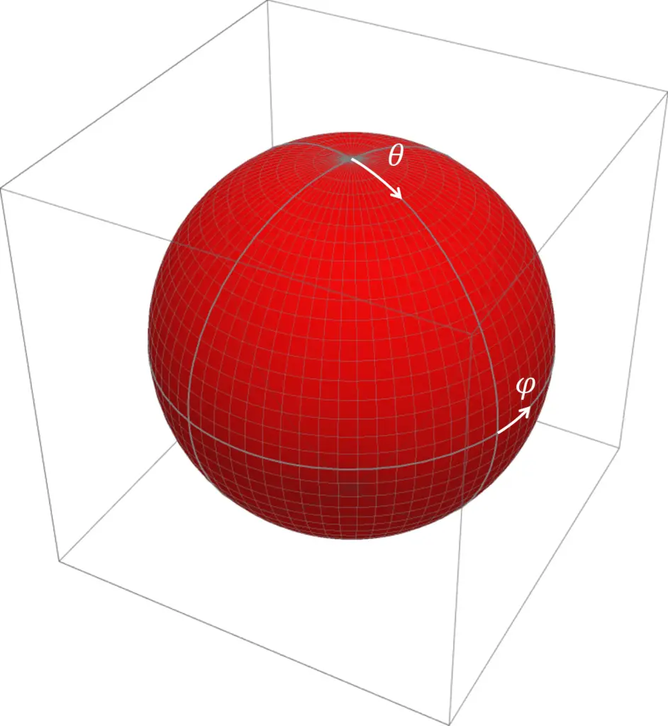
We begin by writing a point on the unit sphere as$$
P(\theta,\varphi)=(\sin\theta\cos\varphi,\ \sin\theta\sin\varphi,\ \cos\theta)
$$where \(\theta\) is the colatitude measured from the north pole and \(\varphi\) is the longitude. The line element \(\delta s\) on the sphere (i.e., the distance from \(P(\theta,\varphi)\) to \(P(\theta+\delta\theta,\varphi+\delta\varphi)\)) is$$
\delta s^2=\delta\theta^2+\sin^2\theta\,\delta\varphi^2
$$and the area element \(\delta S\) (i.e., the area of the infinitesimal region with \(P(\theta,\varphi)\) as one vertex, bounded by coordinate lines of \(\theta\) and \(\varphi\)) is$$
\delta S=\sin\theta\,\delta\theta\,\delta\varphi
$$
Now consider projecting a point on the unit sphere onto a point inside a circle on a plane. For an azimuthal projection centered at the pole, it is natural to identify the azimuthal angle on the plane with the longitude \(\varphi\) on the sphere, and there is no compelling reason to adopt any other convention. Therefore, the essence of the projection lies in how to map the colatitude \(\theta\) on the sphere to the radius \(r\) on the plane.
Let us assume that the spherical coordinates \(P(\theta,\varphi)\) are transformed to planar coordinates \((X,Y)\) by the following mapping:$$
(X,Y) = \bigl( r(\theta)\cos\varphi,\ r(\theta)\sin\varphi \bigr)
$$We leave the specific form of \(r(\theta)\) unspecified for the moment, but assume at least that it is a differentiable function. Under these conditions, let us examine the relationship between infinitesimal elements on the sphere and those on the plane.

Condition for Conformal Projection
First, consider a variation along the meridian direction (a change in \(\theta\)). When \(\theta\) changes to \(\theta+\delta\theta\), the change on the sphere is \(\delta\theta\) itself, but on the planar circle the radial change is \( \delta\theta\, \large{\frac{dr}{d\theta}} \). In other words, an infinitesimal change on the sphere is magnified by a factor of \(\large{\frac{dr}{d\theta}} \) on the plane.
On the other hand, the parallel (latitude) direction corresponds to a change in \(\varphi\). When \(\varphi\) changes to \(\varphi+\delta\varphi\), the change on the sphere is \(\sin\theta\, \delta\varphi\), while on the planar circle it becomes \(r\, \delta\varphi\) (note that, unlike the meridian direction, \(\theta\) or \(r\) appears here). Thus, the magnification factor from the sphere to the plane is \(\large{\frac{r}{\sin\theta}}\).
Now, parallels and meridians are always orthogonal, both on the sphere and on the plane. This means that within any infinitesimal region of the sphere or the plane, one can always choose the parallel and meridian directions as axes (basis vectors) of an orthogonal coordinate system. If the ratio of the lengths of these two basis vectors does not change under the projection from sphere to plane, then figures expressed in that coordinate system remain similar (angles are preserved). That is, we conclude that a conformal projection is one that satisfies $$\frac{dr}{d\theta} = \frac{r}{\sin\theta}$$
Condition for Equal-Area Projection
What about areas? As already noted, the area element on the sphere is$$\delta S=\sin\theta\,\delta\theta\,\delta\varphi$$On the other hand, as can be seen from the figure above, the area element \(\delta A\) on the plane can be written as$$\delta A=r\,\delta r\,\delta\varphi=r\, \frac{dr}{d\theta}\,\delta\theta\,\delta\varphi $$An equal-area projection requires that \(\delta A\) be proportional to \(\delta S\), so in short, an equal-area projection is one that satisfies$$
r\,\frac{dr}{d\theta}\propto\sin\theta
$$
Relation to the Jacobian Matrix and Jacobian
Using the concept of the Jacobian explained on the previous page, the quantities \(\frac{dr}{d\theta}\) and \(\frac{r}{\sin\theta}\) introduced above are none other than the stretching factors (singular values) of the Jacobian matrix along its two principal directions for this mapping. The conformal condition means that these two singular values are equal (i.e., the mapping is a local similarity transformation). The equal-area condition, on the other hand, means that the product of the two singular values (= the Jacobian) is constant, i.e., the ratio of the sphere’s area element \(\delta S\) to the plane’s area element \(\delta A\) is the same everywhere.
Each of the projection methods described below is designed so that \(r(\theta)\) satisfies either the conformal or the equal-area condition.
Stereographic Projection (Conformal Projection)
Geometry of Stereographic Projection
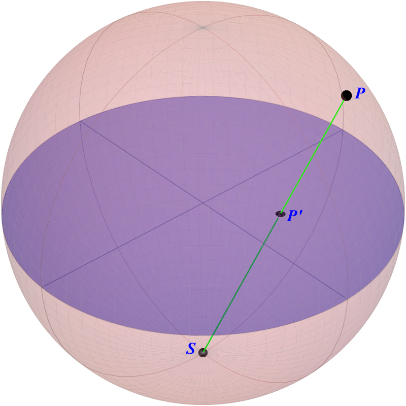
The stereographic projection is a classical projection method used mainly in crystallography and mineralogy. A line is drawn from the south pole \(S=(0,0,-1)\) through a point \(P\) on the sphere, and the intersection \(P’\) with the equatorial plane \(Z=0\) gives the projected point. This projection preserves angles; that is, it maps circles on the sphere to circles (or straight lines) on the plane.
Under this projection, a point \(P = (x,y,z)\) on the sphere is transformed to a point \(P’=(X,Y)\) on the plane as follows:$$(X,Y)=\left(\frac{x}{1+z},\ \frac{y}{1+z}\right)
$$The inverse mapping is$$
(x,y,z)=\frac{1}{1+X^2+Y^2} \left(
2X,\ 2Y,\ 1-X^2-Y^2\right)
$$
Conformality
Let us verify that this projection is indeed conformal by examining the functional form of \(r(\theta)\). Expressing \((X,Y)\) in terms of \(\theta\) and \(\varphi\):$$
(X,Y)=\left(\frac{x}{1+z},\ \frac{y}{1+z}\right)=\left(\frac{\sin\theta\cos\varphi}{1+\cos\theta},\ \frac{\sin\theta\sin\varphi}{1+\cos\theta}\right)=
\left( \tan\frac{\theta}{2}\cos\varphi,\tan\frac{\theta}{2}\sin\varphi \right)
$$so the function \(r_S\) that maps the colatitude \(\theta\) on the sphere to the radius on the plane is$$r_S(\theta)=\tan\frac{\theta}{2}$$As discussed, a conformal projection satisfies \(dr/d\theta = r/ \sin\theta\). We have$$\frac{dr_S}{d\theta}=\frac{1}{2\cos^2\frac{\theta}{2}}
$$while$$
\frac{r_S}{\sin\theta}=\frac{\tan\frac{\theta}{2}}{2\sin\frac{\theta}{2}\cos\frac{\theta}{2}}=\frac{1}{2\cos^2\frac{\theta}{2}}
$$Since \(dr/d\theta = r/ \sin\theta\) holds identically (the radial and azimuthal magnification factors are equal), this projection preserves local angles.
Note that the stereographic projection does not preserve areas. Considering the area element,$$
\delta A=r_S\,r_S'(\theta)\,\delta\theta\,\delta\varphi
=\tan\frac{\theta}{2}\cdot\frac{1}{2}\sec^2\frac{\theta}{2}\,\delta\theta\,\delta\varphi
$$Comparing this with \(\delta S=\sin\theta\,\delta\theta\,\delta\varphi\), we see that the area magnification factor depends on \(\theta\).
Projection of Points with \(Z \lt 0\)
The projection described above can be applied to all points on the sphere except the south pole \(S\), and conformality is maintained throughout. For points on the hemisphere with \(Z \ge 0\), the projected points lie within the unit circle on the plane. However, when projecting points with \(Z \lt 0\), the radial distance on the plane exceeds 1, and for points near \(S\) the projected point lies very far from the center, making graphical representation difficult. For this reason, in standard stereographic projection, one typically either:
- Restricts the points to be projected to those with \(Z \ge 0\)
- For points with \(Z \lt 0\), draws a line from the opposite pole \(N=(0,0,1)\) and takes the intersection with the equatorial plane as the projected point
In the latter case, it is common practice to distinguish the hemispheres by using filled and open circles for the projected points.
Stereonet (Wulff Net)
A diagram in which auxiliary lines such as parallels and meridians are plotted based on the stereographic projection is called a stereonet or Wulff net. It is convenient for reading relative angles between faces and directions, and is well suited for representing crystal morphology and for investigating the orientation relationships of zones and zone axes. On the other hand, when one wishes to compare density or frequency distributions by area, the equal-area projection described next is more natural and useful.

Stereonet (polar center)

Stereonet (equatorial center)
Lambert Azimuthal Equal-Area Projection
Geometry of Lambert Projection
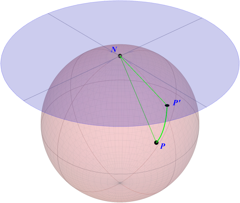
The Lambert azimuthal equal-area projection is an azimuthal projection designed to transfer areas on the sphere faithfully onto the plane. Consider a plane tangent to the sphere at the north pole \(N=(0,0,1)\). Then consider a circle lying in a plane perpendicular to that tangent plane, centered at \(N\) and passing through the point \(P\). The intersection of this circle with the tangent plane gives the projected point \(P’\).
Under this projection, a point \(P=(x,y,z)\) on the sphere is transformed to a point \(P’=(X,Y)\) on the plane as follows:$$
(X,Y)=\left(
\sqrt{\frac{2}{1+z}}\,x,\ \sqrt{\frac{2}{1+z}}\,y \right)
$$Points with \(Z \ge 0\) are mapped inside a circle of radius \(\sqrt{2}\). This circle has the same area as the hemisphere’s surface area. Points on the entire sphere (including \(Z \lt 0\)) are mapped inside a circle of radius \(2\), which has the same area as the total surface area of the sphere.
The inverse mapping of this transformation is as follows:$$
(x,y,z)=\left(
X\sqrt{1-\frac{X^2+Y^2}{4}},\ Y\sqrt{1-\frac{X^2+Y^2}{4}},\ 1-\frac{X^2+Y^2}{2}
\right)$$
Equal-Area Property
Let us verify that this projection indeed has the equal-area property. Expressing \((X,Y)\) in terms of \(\theta\) and \(\varphi\):$$
\left(\sqrt{\frac{2}{1+z}}\,x,\ \sqrt{\frac{2}{1+z}}\,y \right)=
\left(\sqrt{\frac{2}{1+\cos\theta}}\,\sin\theta\cos\varphi,\ \sqrt{\frac{2}{1+\cos\theta}}\,\sin\theta\sin\varphi \right)
$$so the function \(r_L\) that maps the colatitude \(\theta\) on the sphere to the radius on the plane is
$$r_L(\theta)=\sqrt{\frac{2}{1+\cos\theta}}\,\sin\theta=\sqrt{2(1-\cos\theta)}= 2\sin\frac{\theta}{2}
$$and its derivative is$$
\frac{dr_L}{d\theta}=\cos\frac{\theta}{2}
$$Therefore, the area element on the plane is$$
\delta A=r_L\frac{dr_L}{d\theta}\,\delta\theta\,\delta\varphi
=2\sin\frac{\theta}{2}\cos\frac{\theta}{2}\,\delta\theta\,\delta\varphi
=\sin\theta\,\delta\theta\,\delta\varphi
$$The right-hand side is exactly the area element \(\delta S\) of the sphere, so \(\delta A=\delta S\) holds everywhere.
On the other hand, the Lambert projection does not preserve angles. Comparing the magnification factors in the meridian and parallel directions,$$
\frac{dr_L}{d\theta}=\cos\frac{\theta}{2},\qquad
\frac{r_L}{\sin\theta}=\frac{2\sin(\theta/2)}{2\sin(\theta/2)\cos(\theta/2)}=\frac{1}{\cos(\theta/2)}
$$In general \(\cos(\theta/2) \neq 1/\cos(\theta/2)\), so the magnification factors in the two directions do not agree. Therefore, while this projection correctly preserves areas, shapes and angles are distorted.
Schmidt Net
A net based on the Lambert azimuthal equal-area projection is called a Schmidt net. When one needs to compare frequencies per unit solid angle—such as the Orientation Distribution Function (ODF) or the probability distribution of slip directions on faults—the equal-area property is essential, and the Schmidt net is widely used. Note that depending on the field or context, the Schmidt net is sometimes referred to broadly as a “stereonet.”

Schmidt net (polar center)

Schmidt net (equatorial center)
Rosca–Lambert Projection
The projection methods described so far are classical ones found in any textbook. The method described next is a somewhat unusual projection based on relatively recent publications.
The Lambert azimuthal equal-area projection maps points on the hemisphere to the interior of a disc of radius \(\sqrt{2}\). Mapping the sphere to a circle is geometrically natural, but in numerical computation and image processing, grids based on squares or regular hexagons can be more convenient. The Rosca–Lambert equal-area projection is a two-stage construction: first, a polygonal region on the plane is mapped to a disc, and then the inverse Lambert mapping lifts the disc onto the sphere. The key idea of this method is the equal-area transformation from a polygon to a disc on the plane.
Square Grid Version1
Rosca Transform from Square to Disc
First, consider a square whose area equals half the surface area of the unit sphere (\(=2\pi\)):$$
S={(a,b)\in\mathbb{R}^2\mid |a|\le \sqrt{\frac{\pi}{2}},\ |b|\le \sqrt{\frac{\pi}{2}}}
$$and a disc:$$
C={(A,B)\in\mathbb{R}^2\mid A^2+B^2\le 2}
$$

The square Rosca mapping is defined by dividing the square into 8 sector regions. Writing only the representative cases:
Region \(1\): $$(A,B)=\left(\frac{2a}{\sqrt{\pi}}\cos\frac{\pi b}{4a},\ \frac{2a}{\sqrt{\pi}}\sin\frac{\pi b}{4a}\right), \qquad 0<|b|\le |a|\le \sqrt{\pi/2}$$
Region \(2\): $$(A,B)= \left(\frac{2b}{\sqrt{\pi}}\sin\frac{\pi a}{4b},\ \frac{2b}{\sqrt{\pi}}\cos\frac{\pi a}{4b}\right), \qquad0<|a|\le |b|\le \sqrt{\pi/2}$$

Looking at these formulas, we see that whichever of \(|a|\) or \(|b|\) is larger determines the disc radius, and the ratio \(b/a\) or \(a/b\) determines the azimuthal angle. In other words, concentric square layers are rearranged into concentric circles on the disc.
Jacobian of the Square Rosca Transform
Let \(J_{R_T}(a,b)\) denote the Jacobian matrix of the square Rosca transform \((a,b)\to(A,B)\). For Region \(1\), setting \(s=\frac{\pi b}{4a}\), the Jacobian matrix is$$
J_{R_T}(a,b)=\begin{pmatrix}
\frac{2}{\sqrt{\pi}}\cos s+\frac{\sqrt{\pi}b}{2a}\sin s & -\frac{\sqrt{\pi}}{2}\sin s\\[1ex]
\frac{2}{\sqrt{\pi}}\sin s-\frac{\sqrt{\pi}b}{2a}\cos s & \frac{\sqrt{\pi}}{2}\cos s
\end{pmatrix}
$$Computing the determinant yields \(\det J_{R_T}(a,b)=1\). By symmetry, \(\det J_{R_T}=1\) also holds in Region \(2\). Thus the square Rosca transform is an equal-area mapping with Jacobian identically equal to 1 in every region.
Spherical Projection of the Square Grid
Since both the square Rosca transform and the Lambert projection are equal-area mappings, their composition and inverse are naturally also equal-area. The inverse Lambert mapping is$$
(x,y,z)=\left(A\sqrt{1-\frac{A^2+B^2}{4}},\ B\sqrt{1-\frac{A^2+B^2}{4}},\ 1-\frac{A^2+B^2}{2}\right)
$$Composing this with the square Rosca transform, for Region \(1\) we get$$
(x,y,z)= \left(\frac{2a}{\sqrt{\pi}}\sqrt{1-\frac{a^2}{\pi}}\cos\frac{\pi b}{4a},\ \frac{2a}{\sqrt{\pi}}\sqrt{1-\frac{a^2}{\pi}}\sin\frac{\pi b}{4a},\ 1-\frac{2a^2}{\pi}\right)
$$Similarly, for Region \(2\):$$
(x,y,z)= \left(\frac{2b}{\sqrt{\pi}}\sqrt{1-\frac{b^2}{\pi}}\sin\frac{\pi a}{4b},\ \frac{2b}{\sqrt{\pi}}\sqrt{1-\frac{b^2}{\pi}}\cos\frac{\pi a}{4b},\ 1-\frac{2b^2}{\pi}\right)
$$
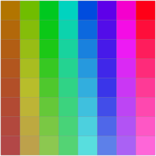
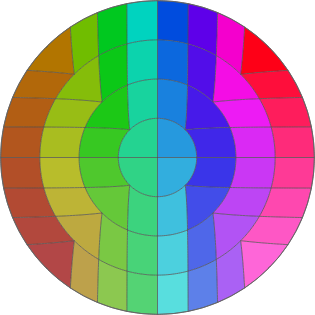
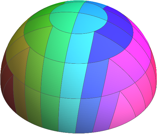
Let us now see how a square grid is actually divided and how each region maps onto the sphere. First, we show a \(3\times3\) square grid, the disc grid obtained via the square Rosca transform, and the result of applying the inverse Lambert mapping to project it onto the sphere.
Square grid \(3\times3\)

Square Rosca transform

Inverse Lambert of the square Rosca transform
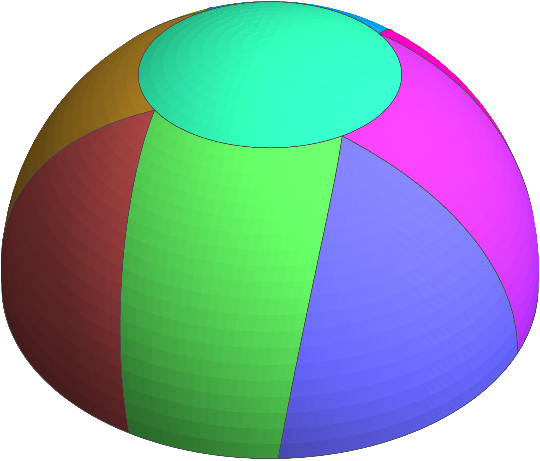
The regions are color-coded to show the correspondence. Squares that overlap with the diagonals are transformed into triangular regions by the square Rosca transform, and the perimeter of the origin-centered square is mapped to parallels (latitude lines). Next, we show the \(8\times8\) case.
Square grid \(8\times8\)
Square Rosca transform
Inverse Lambert of the square Rosca transform
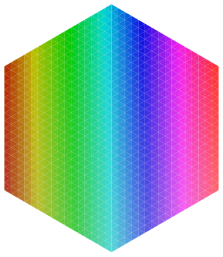
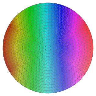
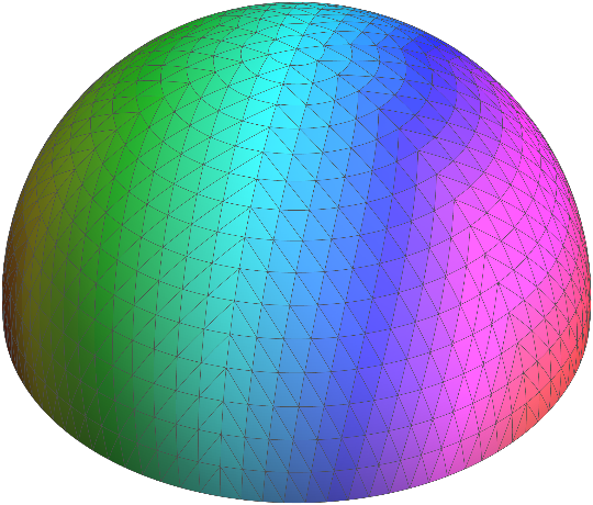
Finally, the \(32\times32=1024\) case.
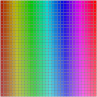
Square grid \(32\times32\)
Square Rosca transform
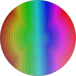
Inverse Lambert of the square Rosca transform
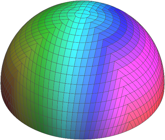
In the usual latitude–longitude grid, the longitude degenerates at the poles, causing coordinate singularities. By contrast, the Rosca–Lambert transform enables the sphere to be handled using a more uniform equal-area partition. Moreover, since the spherical region can be represented as a square array, this approach offers advantages such as easy implementation in programming code and straightforward interpolation. Furthermore, from the crystallographic perspective, when the symmetry of the square grid (i.e., point group \(4/mmm\)) coincides with the symmetry of the crystal under study, the computational domain can be reduced2, leading to a potential reduction in computation time.
Hexagonal Grid Version
While the square Rosca transform is an excellent method, the hexagonal grid may be more advantageous depending on the symmetry of the crystal under study (e.g., trigonal/hexagonal crystal systems). Rosca et al. therefore also constructed an equal-area mapping from a regular hexagon to a disc3.
Mapping from Regular Hexagon to Disc
As in the square grid version, consider a regular hexagon with area equal to half the surface area of the unit sphere (\(2\pi\)). If the inradius of the regular hexagon (area \(2\pi\)) is \(L\), then$$
\frac{6L^2}{\sqrt{3}}=2\pi\quad \to \quad L^2=\frac{\pi}{\sqrt{3}}
$$Next, the hexagon is divided into 12 sector regions (dodecants) as shown in the figure. For example, the points \(a,b\) in Region \(1\) satisfy$$
\left\{(a,b)\in\mathbb{R}^2\ \middle|\ 0\le b\le \frac{a}{\sqrt{3}},\ 0\le a\le L\right\}
$$The hexagonal Rosca transform defines a mapping for each such region.

The mapping for Region \(1\) is defined as$$
(A,B)=\frac{\sqrt{2}\,a}{L}\left(\cos\frac{\pi b}{2\sqrt{3}\,a},\ \sin\frac{\pi b}{2\sqrt{3}\,a}\right)
$$That is, the value of \(a\) maps to the disc radius \(\sqrt{2}\,a/L\), and the slope \(b/a\) maps to the azimuthal angle \(\frac{\pi}{2\sqrt{3}}\cdot\frac{b}{a}\). Region \(12\) is the mirror image of Region \(1\) with respect to the line \(y=0\), and the remaining 10 regions are obtained by rotating these two by \(60^\circ\) increments.
Jacobian Condition for the Hexagonal Version
Let us verify that this mapping is indeed equal-area. Setting \(s=\frac{\pi b}{2\sqrt{3}\,a}\), we have \(A=\frac{\sqrt{2}\,a}{L}\cos s\), \(B=\frac{\sqrt{2}\,a}{L}\sin s\), so the Jacobian matrix is$$
J_{R_H}=\begin{pmatrix}\frac{\partial A}{\partial a} & \frac{\partial A}{\partial b}\\[1ex]\frac{\partial B}{\partial a} & \frac{\partial B}{\partial b}\end{pmatrix}=\frac{\sqrt{2}}{L}\begin{pmatrix}\cos s+\frac{\pi b}{2\sqrt{3}\,a}\sin s & -\frac{\pi}{2\sqrt{3}}\sin s\\[1ex]\sin s-\frac{\pi b}{2\sqrt{3}\,a}\cos s & \frac{\pi}{2\sqrt{3}}\cos s\end{pmatrix}
$$Computing the determinant:$$
\det J_{R_H}=\frac{2}{L^2}\cdot\frac{\pi}{2\sqrt{3}}\bigl(\cos^2 s+\sin^2 s\bigr)=\frac{1}{L^2}\cdot\frac{\pi}{\sqrt{3}}=1
$$By symmetry, \(\det J_{R_H}=1\) also holds in Region \(12\), so the hexagonal Rosca transform is an equal-area mapping with Jacobian identically equal to 1 in all regions.
Spherical Projection of the Hexagonal Grid
Since both the hexagonal Rosca transform and the inverse Lambert mapping are equal-area, their composition is also equal-area. For example, the composite mapping \((a,b)\to(x,y,z)\) for Region \(1\) is$$
(x,y,z)=\left(\frac{\sqrt{2}\,a}{L}\sqrt{1-\frac{a^2}{2L^2}}\cos\frac{\pi b}{2\sqrt{3}\,a},\ \frac{\sqrt{2}\,a}{L}\sqrt{1-\frac{a^2}{2L^2}}\sin\frac{\pi b}{2\sqrt{3}\,a},\ 1-\frac{a^2}{L^2}\right)
$$The formulas for the remaining regions are obtained by applying reflections or reflections combined with rotations to this expression.
Let us look at some concrete examples. For the hexagonal grid, if the number of subdivisions along each edge of the hexagonal domain is \(n\), the total number of cells is \(6n^2\). We show the cases \(n=2\) and \(n=16\).
Hexagonal grid \(n=2\)

Hexagonal Rosca transform
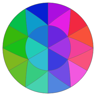
Inverse Lambert of the hexagonal Rosca transform
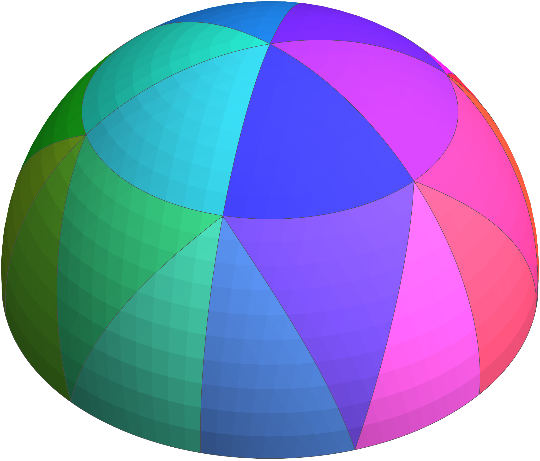
Hexagonal grid \(n=16\)
Hexagonal Rosca transform
Inverse Lambert of the hexagonal Rosca transform
The symmetry of the hexagonal grid is point group \(6/mmm\). This method is well suited when the crystal under study has a common subgroup with this point group.
Features of the Rosca–Lambert Projection
As described above, the Rosca–Lambert projection avoids the gimbal lock problem and provides equal-area coordinates that are compatible with crystal lattices. In particular, the square grid version offers the following advantages:
- Easy implementation using two-dimensional arrays
- Straightforward interpolation
- Good compatibility with point group \(4/mmm\) and its subgroups
The hexagonal grid version partially sacrifices these advantages, but offers:
- Good compatibility with point group \(6/mmm\) and its subgroups
as its own advantage.
Summary
Spherical projection methods are ultimately a question of “which property of the Jacobian matrix do we wish to preserve?”
- The stereographic projection achieves conformality by matching the local magnification factors in the radial and tangential directions
- The Lambert azimuthal equal-area projection achieves equal-area property by keeping the area element constant
- The Rosca–Lambert projection achieves both grid convenience and equal-area property by composing an equal-area mapping from a planar grid region to a disc with the inverse Lambert mapping from disc to sphere
If angular relationships are of primary concern, the Wulff net is appropriate; if comparing areal densities, the Schmidt net is appropriate; and if numerical implementation and compatibility with crystal symmetry are priorities, the Rosca–Lambert representation is effective.
Footnotes
- D. Rosca, “New uniform grids on the sphere”, Astronomy & Astrophysics, 520, A63 (2010). ↩︎
- More precisely, if \(G\) is the largest common subgroup of the crystallographic point group of the crystal under study and \(4/mmm\), then the computational domain of the square grid can be reduced according to the symmetry of \(G\). ↩︎
- D. Rosca and M. De Graef, “Area-preserving projections from hexagonal and triangular domains to the sphere and applications to electron back-scatter diffraction pattern simulations”, Modelling Simul. Mater. Sci. Eng. 21 (2013) 055021. ↩︎