Determinants and the Jacobian

On the previous page, we only stated the conclusions regarding the density distribution of $SO(3)$ in Rodrigues space. Here we explain the concept of the Jacobian that underlies it. In a nutshell, the Jacobian is a quantity that represents “how much an infinitesimal length, area, or volume is scaled up or down by a coordinate transformation.” It becomes easier to understand if you think of it as the multivariable version of the single-variable derivative $dx/dt$.

What Is a Determinant?

Before explaining the Jacobian, let us first review the meaning of the determinant (feel free to skip this section if you don’t need it). A determinant is a scalar quantity defined for a square matrix. Here we consider a $3 \times 3$ matrix$$
M=\begin{pmatrix} a_x & b_x & c_x\\ a_y & b_y & c_y\\ a_z & b_z & c_z\end{pmatrix}
=\left(\begin{array}{c|c|c} & & \\ \mathbf{a} & \mathbf{b} & \mathbf{c}\\ & & \end{array}\right)
$$ $\mathbf{a} , \mathbf{b} , \mathbf{c}$ are 3-dimensional column vectors, but when they appear in the formulas below, please think of them simply as 3-dimensional vectors. The determinant of this matrix is given¹ by $$\det M
=a_x ( b_y c_z-c_y b_z)-b_x (a_y c_z-c_y a_z )+c_x(a_y b_z -b_y a_z )
= \mathbf{a} \cdot (\mathbf{b} \times \mathbf{c}) = \mathbf{b} \cdot (\mathbf{c} \times \mathbf{a}) = \mathbf{c} \cdot (\mathbf{a} \times \mathbf{b})
$$ Here, $\cdot$ denotes the inner product and $\times$ denotes the cross product. Let us consider what this quantity means.

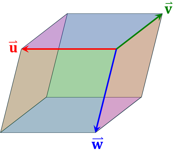
First, given three vectors $ \mathbf{u}, \mathbf{v}, \mathbf{w}$ in 3-dimensional space, the volume $V$ of the parallelepiped they span is²$$
V=\mathbf{u} \cdot (\mathbf{v} \times \mathbf{w})
$$ Now, let $ \mathbf{u}’,\mathbf{v}’,\mathbf{w}’$ be the vectors obtained by applying the linear transformation $M$ to $ \mathbf{u}, \mathbf{v}, \mathbf{w}$. The volume $V’$ of the parallelepiped they span satisfies³$$
V’=\mathbf{u}’ \cdot (\mathbf{v}’ \times \mathbf{w}’)
= [\mathbf{u}\cdot (\mathbf{v} \times \mathbf{w}) ][\mathbf{a} \cdot ( \mathbf{b} \times \mathbf{c}) ]
= V \det M
$$

In other words, the determinant $\det M$ represents the ratio of volume change before and after applying the linear transformation $M$. Note that “volume” should be read as “length” if the matrix dimension is 1, “area” if 2, “volume” if 3, and “hypervolume” if 4 or more.

Note that the sign of $\det M$ contains information about orientation.

$ \det M > 0 $: Preserves orientation (right-handedness/left-handedness)
$ \det M < 0 $: Reverses orientation
$ \det M = 0 $: Collapses along some dimension (volume becomes 0)

When we disregard orientation and consider volume in the usual sense (greater than 0), it is convenient to use the absolute value of the determinant $|\det M|$. Furthermore, basic properties of the determinant include:$$
\det (I) = 1, \quad
\det (AB) = \det (A) \det (B), \quad
\det (A^{-1}) = \{\det (A)\}^{-1}, \quad
\det (A^{\mathrm{T}}) = \det (A)
$$Here, $A^{\mathrm{T}}$ is the transpose of $A$, and $I$ is the identity matrix. The derivations are straightforward, so we omit them.

What Is an Orthogonal Matrix?

This is a slight digression, but the concept of an orthogonal matrix is one you should understand together with the determinant. If $\det M = \pm1$, volume is preserved, but distances and angles are not necessarily preserved. For example,$$
M=\begin{pmatrix} 2 & 0 & 0\\ 0 & 1/2 & 0 \\ 0 & 0 & 1 \end{pmatrix}
$$has $\det M =1$, but it should be immediately clear that this transformation does not preserve distances. So what kind of matrix preserves distances and angles? That is an orthogonal matrix. It is defined for real matrices⁴ and satisfies the following property:$$
M M^{\mathrm{T}} = M^{\mathrm{T}} M =I
$$This condition is equivalent to the following:$$
\mathbf{a} \cdot \mathbf{a} =\mathbf{b} \cdot \mathbf{b}=\mathbf{c} \cdot \mathbf{c}=1 \quad \& \quad
\mathbf{a} \cdot \mathbf{b} =\mathbf{b} \cdot \mathbf{c}=\mathbf{c} \cdot \mathbf{a}=0
$$In other words, it is a matrix where $\mathbf{a}, \mathbf{b}, \mathbf{c}$ are unit vectors that are mutually orthogonal. An orthogonal matrix $M$ always has $\det R = \pm1$⁵. Rotation operations are orthogonal matrices with determinant 1 and preserve not only lengths and angles but also orientation. On the other hand, reflection, inversion, and rotoinversion operations are orthogonal matrices with determinant −1, so they preserve lengths and angles but not orientation.

What Is a Gram Matrix?

A Gram matrix is defined as follows: given an $m \times n$ matrix $M$ and its conjugate transpose⁶ $M^*$, it is the matrix$$G=M^* M$$$G$ is a Hermitian matrix⁷, since $G=M^* M=(M M^*)^*$. Any matrix can be converted into a square one, making this a useful concept in various situations. Note that since we will be considering real matrices from here on, we set $M^*=M^{\mathrm{T}}$.

Let us look at where Gram matrices are used. For example, suppose we have two vectors in 3-dimensional space:$$
\mathbf{u} = (u_x, u_y, u_z),\quad \mathbf{v} =(v_x,v_y,v_z)
$$ Arranging these as columns, we define a $3 \times 2$ matrix: $$
M = \left(\begin{array}{c|c} u_x& v_x\\ u_y & v_y\\ u_z& v_z\end{array}\right)=
\left(\begin{array}{c|c} & \\ \mathbf{u} & \mathbf{v}\\ & \end{array}\right)
$$
The Gram matrix of this is$$
G=M^{\mathrm{T}} M = \left(\begin{array}{ccc} & \mathbf{u} & \\ \hline & \mathbf{v} & \end{array}\right) \left(\begin{array}{c|c} & \\ \mathbf{u} & \mathbf{v}\\ & \end{array}\right)
=\left(\begin{array}{cc} \mathbf{u}^2 & \mathbf{u}\mathbf{v} \\ \mathbf{u}\mathbf{v}&\mathbf{v}^2 \end{array}\right)
$$and its determinant is:$$\begin{array}{l}
\det G = \mathbf{u}^2\ \mathbf{v}^2 – (\mathbf{u}\mathbf{v})^2 \\
\qquad = (u_x^2+ u_y^2+ u_z^2)(v_x^2+ v_y^2+ v_z^2)-(u_xv_x+ u_y v_y+ u_z v_z)^2 \\
\qquad = (u_xv_y-u_yv_z)^2 + (u_yv_z -u_zv_y)^2 + (u_zv_x+u_xv_z)^2 \\
\qquad = (\mathbf{u} \times \mathbf{v} )^2
\end{array}$$A beautiful relationship emerges. That is, the determinant of the Gram matrix generated from two vectors in 3-dimensional space corresponds to the square of the area of the parallelogram spanned by those two vectors. Generalizing further, we have the following result: Choose $n\, (\le m)$ vectors from $m$-dimensional space, form the $m \times n$ matrix $M$ with these as columns, and let the Gram matrix be $G=M^*M$. Then $\det G$ equals the square of the volume spanned by those $n$ vectors. Note that “volume” should be read as “length” if $n$ is 1, “area” if 2, “volume” if 3, and “hypervolume” if 4 or more.

What Is the Jacobian?

Consider a general (not necessarily linear) coordinate transformation of 3 variables: $ (u,v,w)=f(x,y,z) $. That is,$$u=u(x,y,z),\qquad v=v(x,y,z),\qquad w=w(x,y,z)$$The $3\times 3$ matrix formed by arranging the partial derivatives of each component, $$J=\frac{\partial(u,v,w)}{\partial(x,y,z)}=
\large{ \begin{pmatrix}
\frac{\partial u}{\partial x} & \frac{\partial u}{\partial y} & \frac{\partial u}{\partial z}\\
\frac{\partial v}{\partial x} & \frac{\partial v}{\partial y} & \frac{\partial v}{\partial z}\\
\frac{\partial w}{\partial x} & \frac{\partial w}{\partial y} & \frac{\partial w}{\partial z}
\end{pmatrix}}
$$is called the Jacobian matrix, and its determinant $\det J$ is called the Jacobian (Jacobian determinant). The Jacobian matrix is the matrix of the linear transformation obtained by first-order approximation of the coordinate transformation in the neighborhood of point $(x,y,z)$. Therefore, the infinitesimal volume in the neighborhood of $(x,y,z)$ transforms as$$
du\,dv\,dw=\left|
\det\left(\frac{\partial(u,v,w)}{\partial(x,y,z)}\right)
\right| dx\,dy\,dz $$ (the absolute value is taken because volume is non-negative). In other words, the Jacobian represents the rate of change of volume in the neighborhood when the point $(x,y,z)$ is mapped to $(u,v,w)$. Exactly the same approach can be used for transforming probability densities. For example, if we let $p(x,y,z)$ be the density in $(x,y,z)$ space and $p'(u,v,w)$ be the density in $(u,v,w)$ space, then
$$ p(x,y,z)\,dx\,dy\,dz = p'(u,v,w)\,du\,dv\,dw $$ gives us$$
p(x,y,z)= p'(f(x,y,z)) \left| \det\left(\frac{\partial(u,v,w)}{\partial(x,y,z)}\right) \right|
$$The discussion from two pages ago — “uniform on $S^3$, but not uniform in Rodrigues space” — is precisely this density transformation problem.

Jacobian of Polar Coordinates

Consider 3-dimensional spherical coordinates. As on the Spherical Geometry page, let the colatitude be $\varphi$, and the distance from the center be $r$:$$
x=r \sin\theta\cos\varphi,\qquad
y=r \sin\theta\sin\varphi,\qquad
z=r \cos\theta
$$Regarding this as a coordinate transformation $(r,\theta,\varphi)=f(x,y,z)$, the Jacobian matrix is$$
J=\frac{\partial(x,y,z)}{\partial(r,\theta,\varphi)}=\begin{pmatrix}
\sin\theta\cos\varphi & r\cos\theta\cos\varphi & -r\sin\theta\sin\varphi\\
\sin\theta\sin\varphi & r\cos\theta\sin\varphi & r\sin\theta\cos\varphi\\
\cos\theta & -r\sin\theta & 0 \end{pmatrix}
$$and$$
\left| \det J \right| = r^2\sin\theta
$$Therefore, the volume element is$$
dx\,dy\,dz = r^2\sin\theta\,dr\,d\theta\,d\varphi
$$Furthermore, on the unit sphere with $r=1$, the area element is$$
dS=\sin\theta\,d\theta\,d\varphi
$$The appearance of $\sin\theta$ in the area integrals for the spherical cap and spherical triangle on the Spherical Geometry page corresponds to this Jacobian.

Jacobian of Unit Quaternions and Rodrigues Space

Now we come to the main topic. Consider the mapping from Rodrigues coordinates $\mathbf{r}=(x,y,z)$ to unit quaternions $q=(s,\mathbf{v}) =(s,v_x,v_y,v_z) $. Naturally, $s,v_x,v_y,v_z$ are functions of $(x,y,z)$. Letting $\sqrt{x^2+y^2+z^2} = \|\mathbf{r}\|=\rho$, we have$$
s = \frac{1}{\sqrt{1+\rho^2}} , \quad v_x=s\, x, \quad v_y=s\, y, \quad v_z=s\, z
$$(see here for details). This mapping is $\mathbb{R}^3 \to \mathbb{R}^4$, and moreover its image is restricted to $S^3$. Therefore, one cannot simply use the $3\times 3$ Jacobian directly. This is where the Gram matrix comes in handy.

First, let $J$ be the following $4\times 3$ matrix:$$J=\Large{\begin{pmatrix}
\frac{\partial s}{\partial x} & \frac{\partial s}{\partial y} & \frac{\partial s}{\partial z}\\
\frac{\partial v_x}{\partial x} & \frac{\partial v_x}{\partial y} & \frac{\partial v_x}{\partial z}\\
\frac{\partial v_y}{\partial x} & \frac{\partial v_y}{\partial y} & \frac{\partial v_y}{\partial z}\\
\frac{\partial v_z}{\partial x} & \frac{\partial v_z}{\partial y} & \frac{\partial v_z}{\partial z}
\end{pmatrix}}
$$This matrix describes how the displacement changes when a point $(x,y,z)$ in Rodrigues space is shifted by an infinitesimal amount $(dx,dy,dz)$ and mapped to $S^3$. In essence, it is the linear transformation matrix obtained by first-order approximation in the neighborhood of $(x,y,z)$. On the other hand, as explained in the Gram matrix section, it can also be viewed as a matrix with three vectors from 4-dimensional space arranged as columns. Following the latter interpretation, the volume spanned by these three vectors is given by $$
\sqrt{\det(J^*J)}
$$and this quantity represents how much the infinitesimal volume $d^3\mathbf{r}=dx\ dy\ dz$ in the neighborhood of $(x,y,z)$ in Rodrigues space changes on $S^3$ (i.e., the rate of change).

Let us now actually compute $\det(J^*J)$. First, evaluating the partial derivatives of each component of $J$, we get$$
J= \begin{pmatrix}
-s^3 x & -s^3 y & -s^3 z\\ s-s^3x^2 & -s^3 xy & -s^3zx\\ -s^3xy&s-s^3y^2 & -s^3yz\\ -s^3zx & -s^3yz & s-s^3z^2
\end{pmatrix}
=s^3 \begin{pmatrix}
-x & -y & -z\\ 1+y^2+z^2 & -xy & -zx\\ -xy&1+z^2+x^2 & -yz\\ -zx & -yz & 1+x^2+y^2
\end{pmatrix}
= s^3 \left(\begin{array}{c|c|c} & & \\ \mathbf{q}_x & \mathbf{q}_y & \mathbf{q}_z\\ & &
\end{array}\right)
$$For the vectors $\mathbf{q}_x , \mathbf{q}_y , \mathbf{q}_z $ defined at the end, we easily obtain relationships such as$$
\mathbf{q}_x \cdot \mathbf{q}_x = \frac{1+y^2+z^2}{s^2}, \quad
\mathbf{q}_x \cdot \mathbf{q}_y = -\frac{xy}{s^2}
$$and so the Gram matrix $G$ of $J$ is$$
G=J^*J = s^6 \left(\begin{array}{ccc} & \mathbf{q}_x & \\ \hline & \mathbf{q}_y & \\ \hline &\mathbf{q}_z &
\end{array}\right) \left(\begin{array}{c|c|c} & & \\ \mathbf{q}_x & \mathbf{q}_y & \mathbf{q}_z\\ & &
\end{array}\right)\\
=s^4 \begin{pmatrix}
1+y^2+z^2 & -xy & -zx\\ -xy & 1+z^2+x^2 & -yz \\ -zx & -yz & 1+x^2+y^2
\end{pmatrix}
$$It turns out to have the same form as the lower portion of $J$⁸. We want to find the determinant of this Gram matrix $G$, and since $G$ can be rearranged as $$
G = s^4[ (1+x^2+y^2+z^2) I – \mathbf{r}\ \mathbf{r}^*)] =s^4[ (1+\|r\|^2) I – \mathbf{r}\ \mathbf{r}^*)] = s^2 ( I – s^2\mathbf{r}\ \mathbf{r}^*)
$$⁹ (where $I$ is the $3 \times 3$ identity matrix, $\mathbf{r}=(x,y,z)$ is a column vector, and $\mathbf{r}^*$ is a row vector), we can use the formula known as the matrix determinant lemma¹⁰ to obtain$$
\det G = \det[s^2 ( I – s^2\mathbf{r}\ \mathbf{r}^*)] = (s^2)^3 \det(I) (1-s^2\mathbf{r}^* I \ \mathbf{r}) = s^8
$$Remarkably, we arrive at an extremely simple answer. That is, the infinitesimal volume $d^3 \mathbf{r} = dx\ dy\ dz$ in Rodrigues space changes on $S^3$ by a factor of $$
\sqrt{\det G}=s^4=\frac{1}{(1+\rho^2)^2}
$$ The uniform volume element on $S^3$ (i.e., the volume element corresponding to the Haar measure of $SO(3)$) $d\mu$, when written in Rodrigues coordinates $\mathbf{r}$, becomes$$
d\mu \propto \frac{1}{(1+\rho^2)^2}\,d^3\mathbf{r}
$$Therefore, the density function is also$$
P(\rho) \propto \frac{1}{(1+\rho^2)^2}
$$and normalizing this yields the formula stated on the Rodrigues Space page.

Footnotes

In general, the determinant of an $n \times n$ matrix $A$ (with components $a_{ij}$) is given by$$
\det A=\sum_{\sigma\in S_n} s(\sigma)\prod_{i=1}^{n} a_{i,\sigma(i)}
$$where $S_n$ is the set of all permutations of $\{1,2,..,n\}$ ($n!$ elements), $\sigma$ is one such permutation, and $s(\sigma)$ is 1 if the permutation is even and −1 if odd. ↩︎
The magnitude of $\mathbf{v} \times \mathbf{w}$ corresponds to the area of the parallelogram formed by $\mathbf{b}$ and $\mathbf{c}$, and its direction coincides with the normal to the parallelogram. The inner product of the unit normal vector of the parallelogram with $\mathbf{u}$ corresponds to the height of the parallelepiped when the parallelogram is taken as the base. Therefore, the volume $V= \mathbf{u} \cdot (\mathbf{v} \times \mathbf{w})$ is obtained. ↩︎
Let us expand this carefully. The three vectors before the transformation $\mathbf{u},\mathbf{v},\mathbf{w}$ are$$
\mathbf{u} = (u_x, u_y, u_z),\quad \mathbf{v} =(v_x,v_y,v_z),\quad \mathbf{w}=(w_x,w_y,w_z)
$$The vectors after the transformation $ \mathbf{u}’,\mathbf{v}’,\mathbf{w}’$ are$$
\mathbf{u}’ = u_x \mathbf{a} +u_y \mathbf{b} +u_z \mathbf{c}, \quad
\mathbf{v}’ = v_x \mathbf{a} +v_y \mathbf{b} +v_z \mathbf{c}, \quad
\mathbf{w}’ = w_x \mathbf{a} +w_y \mathbf{b} +w_z \mathbf{c}
$$The volume $V’$ of the parallelepiped they span, using the relations $\mathbf{a}\times \mathbf{a}=0,\ \mathbf{a}\times \mathbf{b}=-\mathbf{b}\times \mathbf{a},\ \mathbf{a} \cdot (\mathbf{a}\times \mathbf{b})=0$, is$$\begin{array}{l}
V’=\mathbf{u}’ \cdot (\mathbf{v}’ \times \mathbf{w}’)\\
\qquad = (u_x \mathbf{a} +u_y \mathbf{b} +u_z \mathbf{c}) \cdot
[ (v_x \mathbf{a} +v_y \mathbf{b} +v_z \mathbf{c}) \times (w_x \mathbf{a} +w_y \mathbf{b} +w_z \mathbf{c} ) ]\\
\qquad =(u_x \mathbf{a} +u_y \mathbf{b} +u_z \mathbf{c}) \cdot
[ (w_y v_x -w_x v_y) \mathbf{a} \times \mathbf{b} + (v_y w_z -v_z w_y ) \mathbf{b} \times \mathbf{c} + (v_z w_x -v_x w_z ) \mathbf{c} \times \mathbf{a} ]\\
\qquad =u_x (v_y w_z -v_z w_y )\ \mathbf{a} \cdot ( \mathbf{b} \times \mathbf{c})
+u_y (v_z w_x -v_x w_z )\ \mathbf{b} \cdot ( \mathbf{c} \times \mathbf{a})
+u_z (w_y v_x -w_x v_y)\ \mathbf{c} \cdot ( \mathbf{a} \times \mathbf{b}) \\
\qquad = [u_x (v_y w_z -v_z w_y ) + u_y (v_z w_x -v_x w_z ) +u_z (v_x w_y -v_y w_x) ]\ \mathbf{a} \cdot ( \mathbf{b} \times \mathbf{c}) \\
\qquad = [\mathbf{u}\cdot (\mathbf{v} \times \mathbf{w}) ][\mathbf{a} \cdot ( \mathbf{b} \times \mathbf{c}) ]
\end{array}$$ ↩︎
For matrices with complex components, the generalization of orthogonal matrices is called a unitary matrix. That is, a square complex matrix $M$ satisfying$$
M M^* = M^* M =I$$ ↩︎
Because $\det(R^\textrm{T} R) = \det(R^\textrm{T}) \det(R) = \{\det(R)\}^2 = \det(I) =1$. ↩︎
A matrix obtained by taking the complex conjugate of all components and then transposing. For real matrices, it is simply the transpose. ↩︎
A matrix whose conjugate transpose equals itself. For real matrices, this is a symmetric matrix. ↩︎
This is of course no coincidence. Removing the coefficient $s^3$ from $J$ and rewriting as $$
J’=\begin{pmatrix}-x & -y & -z\\ 1+y^2+z^2 & -xy & -zx\\ -xy&1+z^2+x^2 & -yz\\ -zx & -yz & 1+x^2+y^2\end{pmatrix}=
\begin{pmatrix} & -\mathbf{r}^* &\\ \hline & & \\ & \Large{A} & \\ & & \end{pmatrix}
$$Here, $A$ is a symmetric matrix, $\mathbf{r}=(x,y,z)$ is a column vector, and $\mathbf{r}^*$ is a row vector. The Gram matrix $G$ is$$
G=J’^* J’ =
\left( \begin{array}{c|ccc} & & & \\ -\mathbf{r} & & \Large{A} & \\ & & & \end{array}\right)
\begin{pmatrix} & -\mathbf{r}^* &\\ \hline & & \\ & \Large{A} & \\ & & \end{pmatrix}=
\mathbf{r}\mathbf{r}^*+A^2
$$Also, $A$ can be written as$$A = (1+x^2+y^2+z^2) I – \mathbf{r}\ \mathbf{r}^*= (1+\rho^2) I – \mathbf{r}\ \mathbf{r}^*$$(see the next footnote), so noting that $ (\mathbf{r}\ \mathbf{r}^*)^2 = \mathbf{r}(\mathbf{r}^*\ \mathbf{r}) \mathbf{r}^* = \rho^2 \mathbf{r}\ \mathbf{r}^*$, $A^2$ is$$
A^2 = (1+\rho^2)^2 I^2 – 2 (1+\rho^2) I \mathbf{r}\ \mathbf{r}^* + (\mathbf{r}\ \mathbf{r}^*)^2 =
(1+\rho^2)^2 I -(2+\rho^2)\mathbf{r}\ \mathbf{r}^*
$$Substituting this into $G$ gives$$
G=\mathbf{r}\mathbf{r}^* + (1+\rho^2)^2 I -(2+\rho^2)\mathbf{r}\ \mathbf{r}^* =
(1+\rho^2) [(1+\rho^2)I- \mathbf{r}\ \mathbf{r}^*] =(1+\rho^2) A
$$That is, $G$ is $1+\rho^2$ times $A$. ↩︎
In general, such matrix operations are called rank-1 updates. That is, for a square matrix $A$ and two column vectors $\mathbf{u}, \mathbf{v}$, the operation is$$
A’ = A+ \mathbf{u} \mathbf{v}^*
$$If $A’$ is a symmetric matrix and for some scalar $\sigma$, the rank of $A’ -\sigma I$ is at most 1, then necessarily$$
A’ = \sigma I+ \mathbf{u} \mathbf{u}^*
$$ ↩︎
Though presented somewhat ad hoc, for a square matrix $A$ and column vectors $\mathbf{u},\mathbf{v}$ of the same dimension, there exists the formula$$
\det (A+\mathbf{u} \mathbf{v}^*) =(1+\mathbf{v}^* A \mathbf{u} ) \det(A)
$$This is called the matrix determinant lemma. ↩︎