2.0. Overview
Clicking the “Profile Information” icon or checking its checkbox in the Main Window opens the following window. This window allows you to configure detailed settings for profiles.
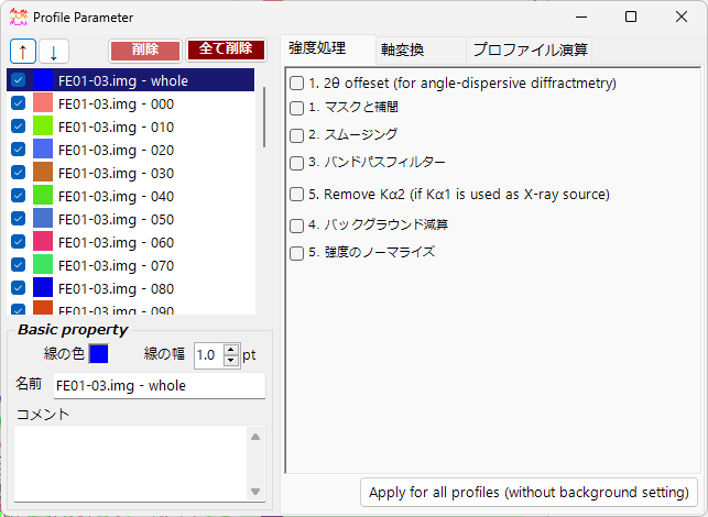
2.1. Profile List
This displays the same information as the profile list in the Main Window.
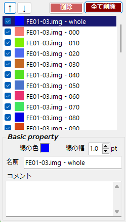
Up/Down Arrow Buttons
Changes the order of profiles.
Delete Button
Deletes the selected profile.
Delete All Button
Deletes all profiles.
Line Color
Click to change the drawing color of the profile selected in the list.
Line Width
Sets the line thickness of the profile.
Name
Sets the name of the profile.
Comment
A free-form comment field.
2.2. Profile Processing
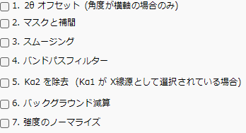
Provides various processing functions for the selected profile.
Checking each item reveals its detailed settings. Processing is applied in order from 1 to 7.
1. 2θ Offset
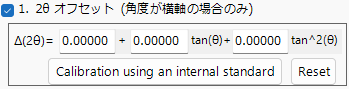
Applies angular correction to angle-dispersive data. The correction formula is a quadratic function of tan(θ). For profiles containing an internal standard sample (i.e., a sample with known lattice parameters), pressing the “Calibration using an internal standard” button and following the instructions will automatically determine the quadratic coefficients.
2. Masking and Interpolation
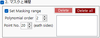
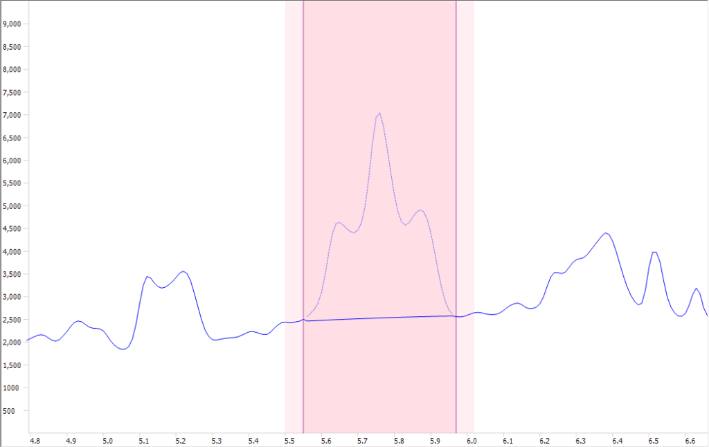
Masks a specified angular range (or energy range) and interpolates the masked region using information from both sides. This is useful when unintended spikes appear in the profile.
With “Set Masking Range” checked, left-dragging in the Main Window adds a mask range (dark pink). On both sides, a range (light pink) with the width specified by “Point No.” is also displayed. The intensity distribution within the light pink range is used to interpolate the masked region. The interpolation function is an n-th order polynomial, and its order is specified by “Polynomial order.”
To delete an added region, press the “Delete” or “Delete all” button.
3. Smoothing
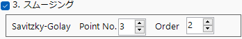
Applies smoothing to the selected profile. The smoothing algorithm is the Savitzky–Golay method1.
4.Bandpass filter
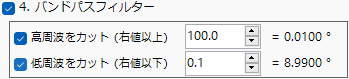
Applies a Fourier transform to the selected profile, cuts components above or below a specified frequency, and then applies an inverse Fourier transform.
5. Remove Kα2

If the X-ray source of the selected profile does not separate Kα1 and Kα2, and it was loaded with Kα1 specified, checking this option removes the diffraction intensity contributed by Kα2.
6. Background
Performs background subtraction.
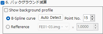
B-spline curve
Pressing “Auto detect” automatically calculates and subtracts the background. Set the maximum number of background control points to search for automatically using “Point No.” You can also manually adjust the background control points. Drag the circular control points drawn on the main screen with the mouse to create an appropriate curve.
Reference
You can specify another profile as the background for the selected profile.
7. Normalize intensity
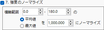
Normalizes the profile so that the average value or maximum value within a specified horizontal axis range equals a specified intensity.
Apply to All Profiles Button
Applies the settings from steps 1 through 7 (excluding 6. Background) to all profiles.
2.3. Axis Conversion
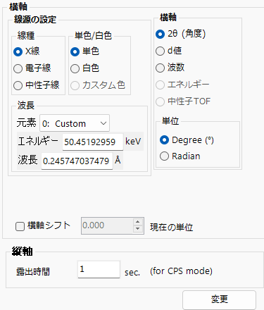
Changes the intrinsic information of the selected profile (units, type of incident radiation, incident radiation energy, etc.). This function is used when you want to modify the horizontal axis or axis information that should have been set when the profile was originally loaded.
The Main Window also has a function to change the horizontal axis, but that only changes the axis for screen display purposes and does not modify the profile’s intrinsic information.
2.4. Profile operator
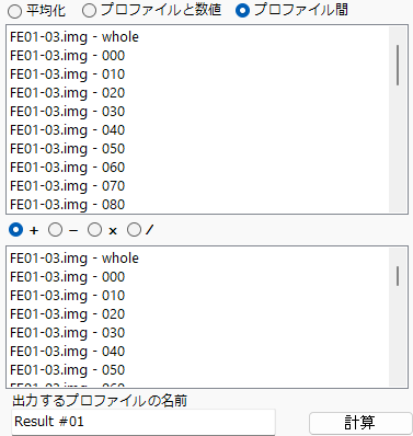
Performs averaging of multiple profiles and arithmetic operations between profiles.
After specifying the target profiles and the desired operation, pressing the “Calculate” button outputs the result as a new profile.
The output profile name defaults to “Result # 01,” but it can be changed.