7.0. Overview
The HRTEM/STEM simulator simulates lattice images obtained by (S)TEM for any crystal and any orientation specified in the main window. It is also possible to simulate potentials.
Click the Simulate button in the lower right to execute the simulation.
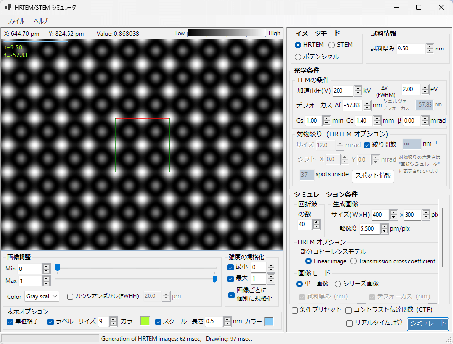
7.1. Main Area
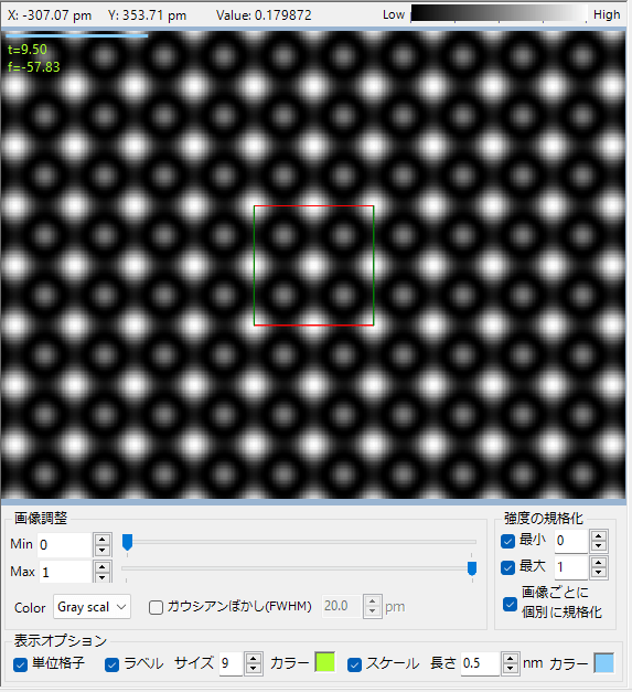
The image obtained from the simulation is displayed.
7.1.1. Mouse Operations
Right-drag to zoom in on a selected area, and right-click to zoom out.
7.1.2. Image Adjustment
Min/Max
Set the maximum and minimum brightness of the image. You can also adjust using the trackbar.
Color
Select either Gray scale or Cold-Warm scale.
Gaussian Blur
Apply a filter (blur) using a Gaussian function to the image. The blur range is specified in pm (picometers).
7.1.3. Display Options
Unit Cell
Set whether to display the unit cell. When displayed, red corresponds to the a-axis, green to the b-axis, and blue to the c-axis.
Label
Set whether to display the label (t: thickness [nm], f: defocus [nm]), as well as the label size and color.
Scale
Set whether to display the scale, and its length and color.
7.1.4. Intensity Normalization
Normalize the maximum/minimum intensity of the image. When displaying series images (described later), you can choose whether to normalize each image individually.
7.1.5.
7.2. File Menu
7.2.1. File
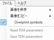
Save the image or copy it to the clipboard. If “Overprint symbols” is checked, the image will be annotated with scale and text information.
7.2.2. Help
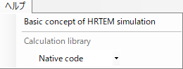
Basic concept of HRTEM simulation
You can view the principles of HRTEM/STEM calculation in a PDF.
Calculation Library
Select the library to use when executing HRTEM/STEM simulation. Native code is usually faster. If Native code does not work, use Managed code instead.
7.3. Image Mode
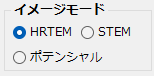
Select either HRTEM mode, STEM mode, or Potential mode. Depending on the selection, the screens displayed in “7.5. Optical Conditions” and “7.6. Simulation Conditions” will change.
7.4. Specimen Information
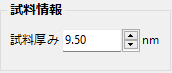
Specimen Thickness
Set the thickness of the specimen. When simulating with “Series Images” (described later), this value is ignored.
7.5. Optical Conditions
Set the observation conditions for the electron microscope.
7.5.1. TEM Conditions
Set parameters specific to the electron microscope. The Scherzer defocus value is displayed based on the accelerating voltage and Cs value. You can also select preset values from the right-click menu.
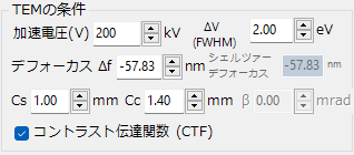
- Accelerating voltage: in kV units
- ΔV: 1/ 𝑒 width of electron energy fluctuations (energy width)
- Defocus Δf: in nm units
- Cs: Spherical aberration coefficient (spherical aberration)
- Cc: Chromatic aberration coefficient (chromatic aberration)
- β: Illumination semi angle due to the finite source size effect (illumination semi-angle)
- Contrast transfer function: displays the contrast transfer function under the set TEM conditions
Right-Click Menu (TEM Conditions)
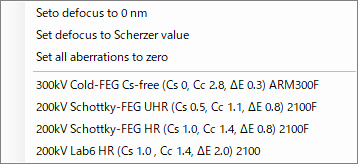
When you right-click in the “TEM Conditions” box, preset TEM conditions are displayed. If you are unsure of your TEM’s condition values, try selecting one that seems similar.
7.5.2 Objective Aperture (HRTEM Option)
Displayed when in HRTEM mode.
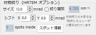
Set the size and position of the objective lens aperture. By launching the “Diffraction Simulator”, you can check the size and position of the aperture.
Size
Set the size of the objective lens aperture in mrad units. To open the aperture fully, check “Aperture open”. Depending on the set aperture conditions, the number of diffraction spots considered in the Bloch wave method changes. The maximum number of spots is limited by the value set in “Number of diffraction waves” (described later).
Shift
Set the horizontal position of the objective lens aperture in mrad units.
Spot Information
Display detailed spot information.
7.5.3. STEM Option
Displayed when in STEM mode. Right-click to display preset values.
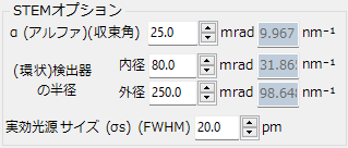
α (Convergence Angle)
Set the angle (semi-angle) of incident electrons in mrad units.
(Annular) Detector Radius
For annular detectors, set the inner and outer diameters. For non-annular detectors (without a central hole), set the inner diameter to zero.
Effective Source Size
Set the source size defined by FWHM in pm units.
Right-Click Menu (STEM Option)
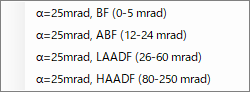
When you right-click in the “STEM Option” box, preset convergence angles and detector radii are displayed. If you are unsure of your STEM’s observation conditions, try selecting one that seems similar.
7.6. Simulation Conditions
7.6.1. Number of Diffraction Waves / Generated Image
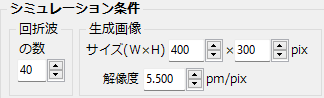
Number of Diffraction Waves
Set the maximum number of Bloch waves included in the calculation. The calculation speed is proportional to the cube of the number of Bloch waves, so large values will take a very long time.
Generated Image
Set the horizontal and vertical pixel count and resolution of the image to be simulated.
7.6.2. HRTEM Option
Displayed when Image Mode is HRTEM.
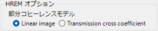
When calculating the HRTEM image, choose whether to calculate the wave interference based on the Linear image model or the Transmission cross coherent model. The latter provides more accurate simulation, but the calculation speed is slower.
7.6.3. STEM Option
Displayed when Image Mode is STEM.
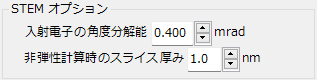
Incident Electron Angular Resolution
In STEM image simulation, like CBED, convergent electrons are considered as a superposition of many plane waves, and the effect of overlapping diffraction disks is calculated. This item sets the angular resolution at which the convergent incident electrons are divided. Naturally, a smaller value improves accuracy but takes more time.
Slice Thickness in Inelastic Calculation
In ReciPro’s algorithm, the specimen is sliced in the thickness direction, and the effect of inelastic electrons is calculated by applying the Riemann sum. This item sets the thickness of the slice. A smaller value improves accuracy but takes more time. Empirically, a thickness of about 1 nm provides sufficient accuracy.
7.6.4. Image Mode
Displayed when Image Mode is HRTEM or STEM.
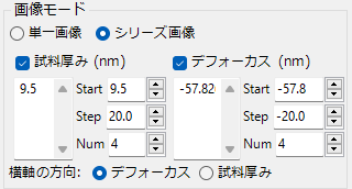
Single Image / Series Image
In single image mode, one image is simulated based on the specimen thickness set in “Specimen Information” and the defocus set in “TEM Conditions“.
In series image mode, images are generated for multiple thicknesses/defoci set by Start/Step/Num.
7.6.5. Potential Option
Displayed when Image Mode is Potential.
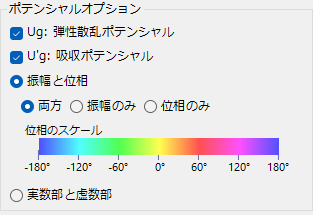
The selected potential (Ug, U’g) becomes the simulation target. Also, select how to display the potential from “Amplitude and phase” or “Real and imaginary parts”.
7.7. Preset, Real-time Calculation, Simulate

7.7.1. Condition Preset
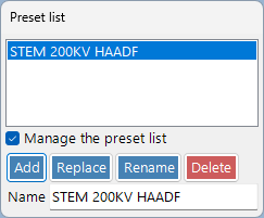
This is a feature that allows you to save and switch between frequently used analysis conditions. All values set in Image Mode, Specimen Information, Optical Conditions, and Simulation Conditions are saved. To add or update a preset, check “Manage the preset list”.
7.7.2. Real-time Calculation
Valid only when Image Mode is HRTEM or Potential. When you rotate the crystal in another window, the HRTEM image or Potential image is calculated and displayed in real-time.
7.7.3. Simulate
Calculate the image with the set condition values. If you want to stop the calculation midway, press the “Cancel” button displayed in the same location.
7.8. Contrast Transfer Function
When you check “Contrast transfer function”, a window like the following opens.
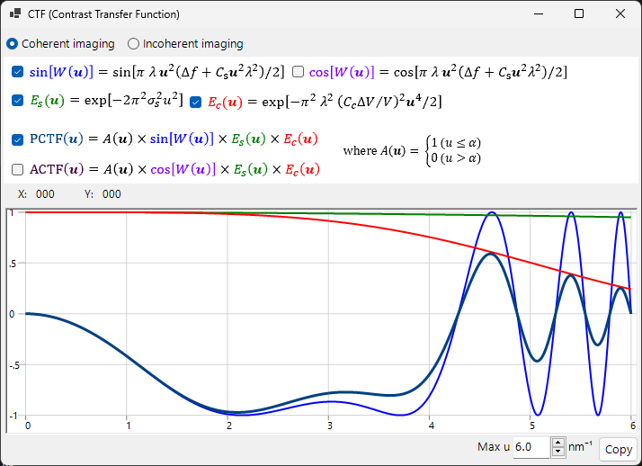
Based on the set TEM conditions (accelerating voltage, aberrations, etc.), it graphs the PCTF (Phase contrast transfer function), ACTF (Amplitude contrast transfer function), and CTFI (contrast transfer function for incoherent imaging, STEM mode only). You can change the drawing range by setting the upper limit of the u value. When you press the “Copy” button, the data is copied in tab-separated format that can be pasted into Excel.